The band theory describes the electronic properties of periodic systems. It calculates the allowed energy states for the electrons within the system. There are two types of bands: the allowed energy bands (valence band & conduction band) and the forbbiden ones (gap). The distribution of this energy bands discriminates materials between, insulators, conductors or semiconductors. To make a band structure calculation, first we have to localize the high symmetry points in the Brillouin Zone of the solid, to study the behaviour of this states.
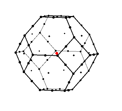
Figure 1. Brillouin Zone of an fcc structure. Made it on Xcrysden .
Band Structure Calculation
After you have an optimized geometry, cell and ions possition, you can perform a Band Structure calculation.
- First You have to perform a single point calculation with very high accuracy on the SCF (electronic relaxation) to
generate the charge distribution on the system (CHG & CHGCAR file).
- Second You perform a single point calculation using this charge distribution to analize the band structure.
Generate the charge density file
Lets build the charge density of the anatase in volume:
- From a converged geometry use the CONTCAR file as POSCAR
- Use the same POTCAR and KPOINTS file.
- To make a single point calculation to you well known INCAR, change the next instructions:
# Anatase volume
#===========================================

# General Setup
  System = Anatase_benz    # Calculation Title
  PREC   = NORMAL     # Options: Normal, Medium, High, Low
  ENCUT  = 400        # Kinetic Energy Cutoff in eV
  ISTART = 0          # Job: 0-new  1-cont  2-samecut
  ICHARG = 2          # initial charge density: 1-file 2-atom 10-cons 11-DOS
  ISPIN  = 1          # Spin Polarize: 1-No 2-Yes

# Electronic Relaxation (SCF)
  NELM     = 150       #Increase the iterations.
    NELMIN = 2        # Min Number of ESC steps
    NELMDL = 10       # Number of non-SC at the beginning
  EDIFF    = 1.0E-05  # Increase the stopping criteria for ESC
  LREAL    = .TRUE.   # Real space projection
  IALGO    = 48       # Electronic algorithm minimization
  VOSKOWN  = 1        # 1- uses VWN exact correlation
  ADDGRID  = .TRUE.   # Improve the grid accuracy

# Ionic Relaxation
  EDIFFG   = 1.0E-04  # Stopping criteria for ionic self cons steps
  NSW      = 0        # Max Number of ISC steps: 0- Single Point
  ISIF     = 2        # Ionic Relaxation
  IBRION     = -1        # Single Point
  ADDGRID  = .TRUE.   # Improve the grid accuracy
  SIGMA    = 0.10     # Insulators/semiconductors=0.1  metals=0.05
  ISMEAR   = 0        # Partial Occupancies for each Orbital
                      # -5 DOS, -2 from file, -1 Fermi Smear, 0 Gaussian Smear
# Parallelization
  NPAR=8
  NCORE=8
This will generate the charge distribution we will use in the next step
Band Structure
Once you have the CHG files you have to make a new calculation:
- Copy the INCAR POTCAR POSCAR CHG and CHGCAR into the new directory.
We are going to scan the next directions of the Brillouin cell:
Kpoints along high symmetry line
 216
line-mode
rec

 0.0  0.0  0.0 ! gamma
 0.0  0.5  0.5 ! X

 0.0  0.5  0.5 ! X
 0.5  0.5  0.5 ! R

 0.5  0.5  0.5 ! R
 0.375 0.75  0.375 ! Z

 0.375 0.75  0.375 ! Z
 0.0  0.0  0.00 ! gamma

 0.0  0.0  0.0 ! gamma
 0.5  0.5  0.0 ! M
- Now we have to add the next instructions to the INCAR:
- ISTART= 1 Job continuation.
- ICHARG= 11 Job continuation.
- ISIF = 2 Ions relaxation.
- IBRION= -1 Single Point
- NSW = 0 Single Point
- LORBIT= 11 Band Structure
- RWIGS = Wigner Seitz atomic radius
# Anatase Bulk Band Structure
#===========================================

# General Setup
  System = Anatase_benz    # Calculation Title
  PREC   = NORMAL     # Options: Normal, Medium, High, Low
  ENCUT  = 400        # Kinetic Energy Cutoff in eV
  ISTART = 1          # Job: 0-new  1-cont  2-samecut
  ICHARG = 11         # Reads the charge distribution to make a BS
  ISPIN  = 1          # Spin Polarize: 1-No 2-Yes

# Electronic Relaxation (SCF)
  NELM     = 150       # More Steps because the criteria
    NELMIN = 2        # Min Number of ESC steps
    NELMDL = 10       # Number of non-SC at the beginning
  EDIFF    = 1.0E-04  # Stopping criteria for ESC
  LREAL    = .TRUE.   # Real space projection
  IALGO    = 48       # Electronic algorithm minimization
  VOSKOWN  = 1        # 1- uses VWN exact correlation
  ADDGRID  = .TRUE.   # Improve the grid accuracy

# Ionic Relaxation
  EDIFFG   = 1.0E-02  # Stopping criteria for ionic self cons steps
  NSW      = 0        # Single Point
  IBRION   = -1       # Single Point
  ISIF     = 2        # Stress and Relaxation: 2-Ion 3-cell+ion
  ADDGRID  = .TRUE.   # Improve the grid accuracy

#BS related values:
  RWIGS  = 1.217 0.820 # Wigner Seits Radius: Ti O
  LORBIT = 11         # Split the bands
  SIGMA    = 0.10     # Insulators/semiconductors=0.1  metals=0.05
  ISMEAR   = 0        # Partial Occupancies for each Orbital
                      # -5 DOS, -2 from file, -1 Fermi Smear, 0 Gaussian Smear
# Parallelization
  NPAR=1
  NCORE=1
Visualizing the Band Structure
To visualize the Band Structure use p4v software. Download the vasprun.xml file into your computer disk, and excecute p4v. There you will find the tools to plot a DOS and the BS
By the end you must have this plot
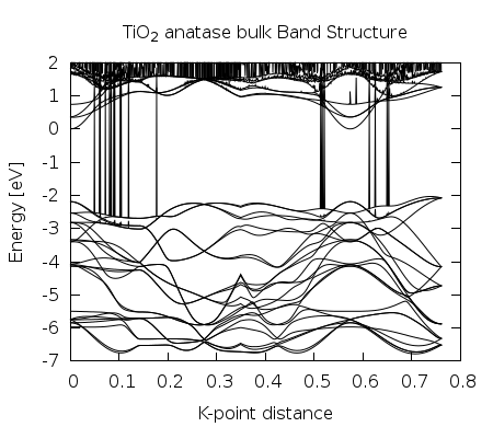
Figure 2. Band Structure generated by Texas utilities and Gnuplot.
You can download the build files here:
INCAR
POTCAR
KPOINTS
POSCAR